Probability Theory

A deterministic model predicts the outcome of an experiment with certainty.

• Velocity of a falling object $v = gt$.

A probabilistic or stochastic model assigns a probability to each possible outcome.

• Rolling a die results in probability of $1/6$.

When there are $N$ possible equally likely outcomes, and $k$ succeses, then the probability is:

$$ P(\text{success}) = \frac{k}{N} $$

These values describe the frequency of the successful outcome and the proportion of times the event occurs in the LONG RUN.

Sample Spaces

The sample space is the set of all possible outcomes of an experiment.

• A discrete sample space has a finite or countably infinite number of elements.

• A continuous sample space is an interval in ℝ.

Individual elements of a sample space are called outcomes while subsets of a sample space are called events.

For example the Probability Spinner has $ \text{Sample space: } {θ \text{ degrees} \mid θ \in [0, 360)}$

Therefore events could be

• Landing between 90 and 180 degrees
  
• Landing either between 45 and 90 degrees or between 270 and 315 degrees
  
• Landing precisely on 180 degrees.

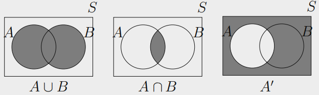
Union, Intersection and Complement

Let $A$ and $B$ be events in sample space $S$

• The Union of $A$ and $B$ is the set of outcomes that are in either $A$ or $B$, or both:

  $$ A ∪ B = { x ∈ S \mid x ∈ A \text{ or } x ∈ B } $$

• The intersection of $A$ and $B$ is the set of outcomes that are in both $A$ and $B$:

  $$ A ∩ B = { x ∈ S \mid x ∈ A \text{ and } x ∈ B } $$

• The Complement of $A$ in $S$ is the set of outcomes in $S$ that are not in $A$:

  $$ A^c = { x ∈ S \mid x \notin A } = S \setminus A $$

A Venn diagram visually represents subsets of a Universal Set $S$

A set with no elements is called the Empty Set, denoted ∅.

Mutually Exclusive Events

Two events are mutually exclusive or disjoint if they cannot occur at the same time for example:

• Event A: Rolling at least one six and Event B: Sum of the dice equals 4

  $$ A = { (d_1, 6), (6, d_2) \mid d_1, d_2 ∈ {1, 2, 3, 4, 5, 6} } $$

  $$ B = { (d, 4-d) \mid d ∈ {1, 2, 3} } $$

The events $A$ and $B$ in this case are called mutually exclusive or disjoint.

Algebra of the Sets

Let $A$, $B$, and $C$ be subsets of a universal set $S$.

Idempotent Laws:
$$ A ∪ A = A, \quad A ∩ A = A $$

Associative Laws:
$$ (A ∪ B) ∪ C = A ∪ (B ∪ C) $$
$$ (A ∩ B) ∩ C = A ∩ (B ∩ C) $$

Commutative Laws:
$$ A ∪ B = B ∪ A $$
$$ A ∩ B = B ∩ A $$

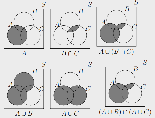
Distributive Laws:
$$ A ∪ (B ∩ C) = (A ∪ B) ∩ (A ∪ C) $$
$$ A ∩ (B ∪ C) = (A ∩ B) ∪ (A ∩ C) $$

Identity Laws:
$$ A ∪ ∅ = A, \quad A ∪ S = S $$
$$ A ∩ S = A, \quad A ∩ ∅ = ∅ $$

Complement Laws:
$$ (A^c)^c = A, \quad A ∪ A^c = S, \quad A ∩ A^c = ∅ $$
$$ S^c = ∅, \quad ∅^c = S $$

De Morgan’s Laws:
$$ (A ∪ B)^c = A^c ∩ B^c $$
$$ (A ∩ B)^c = A^c ∪ B^c $$

We can easily visualize them with Venn Diagrams for example:

$$ A ∪ (B ∩ C) = (A ∪ B) ∩ (A ∪ C) $$

Probability Axioms

Probability must satisfy the following postulates - axioms.

1. Probability Interval: The probability of any event A in sample space is a non-negative ℝ number. Since events can’t happen less than 0% or more than 100%:

$$ 0 \leq P(A) \leq 1, \quad \text{for any event } A $$

2. Sample Space: Since universal set S includes all possible outcomes, the probability of any outcome occurring must:
   $$ P(S) = 1 $$

3. Additivity: If events $A_1, A_2, …$ are mutually exclusive, their total probability is the sum of their individual probabilities: $$ P(A_1 ∪ A_2 \dots) = P(A_1) + P(A_2)\dots $$

Rules

Let $S$ be a sample space with probability measure $P$, and let $A$ and $B$ be events.

1. Complement Rule
   $$ P(A) + P(A^c) = 1, \quad P(A^c) = 1 - P(A) $$

2. Probability of the Empty Set
   $$ P(∅) = 0 $$

3. Subset Rule If A ⊂ B, then:
   $$ P(A) \leq P(B) $$

4. Inclusion-Exclusion for Two Sets
   $$ P(A ∪ B) = P(A) + P(B) - P(A ∩ B) $$

The Inclusion-Exclusion Principle can be generalized to more than two sets.

Conditional Probability

The $P(A|B)$ is called the conditional probability of A given B.

If $A$ and $B$ are events in a sample space, and $P(B) ≠ 0$, then the conditional probability of A given B is defined as:

$$ P(A|B) = \frac{P(A \cap B)}{P(B)} $$

The outcome must lie in both A and B. Therfore, A ∩ B becomes the event of interest, and B is considered the new sample space.

Example:
Consider deck of 52 playing cards. Let A be drawing a King, and B be drawing a Spade.

• $P(A) = 4/52 = 1/13$
• $P(B) = 13/52 = 1/4$
• $P(A ∩ B) = 1/52$

The conditional probability of drawing a King given that the card is a Spade is:

$$ P(A|B) = \frac{P(A \cap B)}{P(B)} = \frac{1/52}{1/4} = \frac{1}{13} $$

Finding Intersections

We can find $P(A ∩ B)$ using the Multiplication Rule of the probability.

$$ P(A \cap B) = P(A) \cdot P(B|A) $$

Imagine selecting two cards from a deck without replacement:

• Let A be the event “the first card is an Ace”.
• Let B be the event “the second card is an Ace”.

1. $P(A)$

   • There are 4 Aces out of 52 cards, so P(A) = 4/52 = 1/13.

2. $P(B|A)$:

   • If the first card was an Ace, there are now 3 Aces left out of 51 cards, so $P(B|A) = 3/51 = 1/17$.

3. Multiply them together: $$ P(A \cap B) = P(A) \cdot P(B|A) = \frac{1}{13} \cdot \frac{1}{17} = \frac{1}{221} $$

Dependent and Independent Events

Independent Events

Two events $A$ and $B$ are said to be independent if the occurrence of one event does not affect the probability of the other event occurring.

$$ P(A|B) = P(A) \quad \text{or} \quad P(B|A) = P(B) $$

The Multiplication Rule for Independent Events is:

$$ P(A \cap B) = P(A) \cdot P(B) $$

Example:
Consider flipping a fair coin and rolling a fair six-sided die.

• Let event A be getting Heads on the coin flip.
• Let event B be rolling a 4 on the die.

Since flipping the coin has no impact on the die roll and vice versa, A and B are independent.

• $P(A) = 1/2$
• $P(B) = 1/6$

The probability of both A and B occurring is:

$$ P(A \cap B) = P(A) \cdot P(B) = \frac{1}{2} \cdot \frac{1}{6} = \frac{1}{12} $$

We can simply multiply the probabilities when events are independent.

Dependent Events

Two events $A$ and $B$ are dependent if the occurrence of one event affects the probability of the other event occurring.

The Multiplication Rule for Dependent Events is:

$$ P(A \cap B) = P(A) \cdot P(B|A) $$

Example:
Consider drawing two cards without replacement from a standard deck of 52 cards.

• Let event A be the first card is a Queen.
• Let event B be the second card is a Queen.

Since the first card is not replaced, the events are dependent because the outcome of the first draw affects the probability of the second draw.

1. $P(A)$: There are 4 Queens in the deck

   $$ P(A) = \frac{4}{52} = \frac{1}{13} $$

2. $P(B|A)$: If the first card was a Queen, there are now 3 Queens left in a deck of 51 cards

   $$ P(B|A) = \frac{3}{51} = \frac{1}{17} $$

3. Joint Probability:

   $$ P(A \cap B) = P(A) \cdot P(B|A) = \frac{1}{13} \cdot \frac{1}{17} = \frac{1}{221} $$

Differences Between Independent and Dependent Events

• Independent Events: The outcome of one event does not influence the outcome of the other.
• Dependent Events: The outcome of one event does influence the outcome of the other.

A quick way to test for independence is to check if:

$$ P(A \cap B) = P(A) \cdot P(B) $$

If this equality holds, the events are independent. If not, the events are dependent.

Bayes’ Theorem

$$ P(A|B) = \frac{P(B|A) \cdot P(A)}{P(B)} $$

Where:

• $P(A|B)$ is the posterior probability
• $P(B|A)$ is the likelihood
• $P(A)$ is the prior probability
• $P(B)$ is the marginal probability

Derivation of Bayes’ Theorem

Derived from the definition of conditional probability:

$$ P(A|B) = \frac{P(A \cap B)}{P(B)} \quad $$

Rearranging the second equation:

$$ P(A \cap B) = P(B|A) \cdot P(A) $$

Substitute this into the first equation:

$$ P(A|B) = \frac{P(B|A) \cdot P(A)}{P(B)} $$

This is Bayes’ Theorem.

Example:

Consider a medical test for a disease:

• $P(Disease)$ = 0.01
• $P(Positive | Disease)$ = 0.99
• $P(Positive | No Disease)$ = 0.05

You receive a positive test result. What is the probability you actually have the disease when the result positive?

1. Calculate $P(Positive)$:

$$ = (0.99 \cdot 0.01) + (0.05 \cdot 0.99) $$

$$ = 0.0099 + 0.0495 = 0.0594 $$

2. Apply Bayes’ Theorem:

$$ \frac{P(Positive|Disease) \cdot P(Disease)}{P(Positive)} $$

$$ = \frac{0.99 \cdot 0.01}{0.0594}\approx \frac{0.0099}{0.0594} \approx 0.1667 $$

So, even with a positive test result, the probability of actually having the disease is approximately 16.67%.

Random Variables

Random Variable is a function that assigns a real number to each outcome of a probability experiment. Usually, capital X used to denote random variables, while their lowercase counterparts x, represent value that X can take. Range is the set of all values a random variable can produce.

Note: A Discrete Random Variable has a countable set of possible values, while a Continuous Random Variable has an uncountable range, covering an interval of real numbers ℝ.

Probability Mass Function

A Probability Mass Function gives the probability of each possible value of a discrete random variable. It tells us how likely each outcome is.

$$ f(x) = P(X = x), \quad \text{where } 0 \leq P(X = x) \leq 1 $$

The total probability of all possible values must sum to 1:

$$ \sum P(X = x) = 1 $$

Finding Probabilities Using the PMF

To find the probability that a discrete random variable equals a specific constant:

$$ P(X = c) = f(c) $$

The probability that the variable falls between two values

$$ P(a \leq X \leq b) = \sum_{x = a}^{b} f(x) $$

$$ P(a < X < b) = \sum_{x = a+1}^{b-1} f(x) $$

Let X be a discrete random variable with PMF:

$$ f(x) = \begin{cases} \frac{1}{8}, & x = 0, \\[6pt] \frac{3}{8}, & x = 1, \\[6pt] \frac{3}{8}, & x = 2, \\[6pt] \frac{1}{8}, & x = 3, \\[6pt] 0, & \text{otherwise}. \end{cases} $$

Therefore the example porbabilities:

$$ P(X = 2) = f(2) = \frac{3}{8} $$

$$ P(1 \leq X \leq 3) = f(1) + f(2) + f(3) = \frac{7}{8} $$

$$ P(0 < X < 3) = f(1) + f(2) = \frac{3}{8} + \frac{3}{8} = \frac{6}{8} = \frac{3}{4} $$

Probability Density Function

A Probability Density Function describes the probability distribution of a continuous random variable. Unlike a PMF, which gives the probability of specific discrete values, the PDF represents probability density over an interval.

For a continuous random variable $X$, the PDF satisfies:

1. Non-negativity: $$ f(x) \geq 0, \quad \forall x \in \mathbb{R} $$

2. Total Probability: $$ \int_{-\infty}^{\infty} f(x) ,dx = 1 $$

3. Probability of a single point $$ P(X = x) = 0 $$

We find probabilities over intervals by integrating within those intervals.

$$ P(a \leq X \leq b) = \int_{a}^{b} f(x) ,dx $$

Note: Whether we use ≤ or < in the bounds does not affect the result, because the probability of a single point is zero.

Cumulative Distribution Function

A Cumulative Distribution Function gives the probability that a random variable $X$ takes on a value less than or equal to a specific value $x$.

$$ F(x) = P(X \leq x) $$

For a discrete random variable, the CDF is the sum of the probabilities of all outcomes less than or equal to $x$:

$$ F(x) = P(X \leq x) = \sum_{t \leq x} P(X = t) $$

• Probability at a constant

$$ P(X = x) = F(x) - F(x - 1) $$

• Probability over an interval

$$ P(a \leq X \leq b) = F(b) - F(a-1) $$

For a continuous random variable, the CDF is the integral of the probability density function from $-∞$ to $x$:

$$ F(x) = P(X \leq x) = \int_{-\infty}^{x} f(t) , dt $$

The derivative of the CDF gives the PDF: $$ f(x) = \frac{d}{dx}F(x) $$

• Probability at a constant value
  $$ P(X = x) = 0 $$

• Probability of an Interval $$ P(a \leq X \leq b) = F(b) - F(a) $$

PMF to CDF Conversion

Consider a discrete random variable X with the following PMF defined over four points:

$$ p(x) = \begin{cases} \frac{1}{8}, & x = 0, \\[6pt] \frac{3}{8}, & x = 1, \\[6pt] \frac{3}{8}, & x = 2, \\[6pt] \frac{1}{8}, & x = 3, \\[6pt] 0, & \text{otherwise}. \end{cases} $$

• For 0 ≤ x < 1:
  $$ F(x) = p(0) = \frac{1}{8} $$

• For 1 ≤ x < 2:
  $$ F(x) = p(0) + p(1) = \frac{1}{8} + \frac{3}{8} = \frac{4}{8} = \frac{1}{2} $$

• For 2 ≤ x < 3:
  $$ F(x) = p(0) + p(1) + p(2) = \frac{1}{8} + \frac{3}{8} + \frac{3}{8} = \frac{7}{8} $$

• For x ≥ 3:
  $$ F(x) = p(0) + p(1) + p(2) + p(3) $$

  $$ = \frac{1}{8} + \frac{3}{8} + \frac{3}{8} + \frac{1}{8} = 1. $$

Therefore the CDF is:

$$ F(x) = \begin{cases} 0, & x < 0, \\[6pt] \frac{1}{8}, & 0 \le x < 1, \\[6pt] \frac{1}{2}, & 1 \le x < 2, \\[6pt] \frac{7}{8}, & 2 \le x < 3, \\[6pt] 1, & x \ge 3. \end{cases} $$

CDF to PMF Conversion

Using the discrete CDF from the previous example:

$$ F(x) = \begin{cases} 0, & x < 0, \\[6pt] \frac{1}{8}, & 0 \le x < 1, \\[6pt] \frac{1}{2}, & 1 \le x < 2, \\[6pt] \frac{7}{8}, & 2 \le x < 3, \\[6pt] 1, & x \ge 3. \end{cases} $$

• For x = 0:
  $$ p(0) = F(0) - \lim_{x \to 0^-} F(x) = \frac{1}{8} - 0 = \frac{1}{8}. $$

• For x = 1:
  $$ p(1) = F(1) - F(0) = \frac{1}{2} - \frac{1}{8} = \frac{3}{8}. $$

• For x = 2:
  $$ p(2) = F(2) - F(1) = \frac{7}{8} - \frac{1}{2} = \frac{3}{8}. $$

• For x = 3:
  $$ p(3) = F(3) - F(2) = 1 - \frac{7}{8} = \frac{1}{8}. $$

Therefore the PMF is:

$$ f(x) = \begin{cases} \frac{1}{8}, & x = 0, \\[6pt] \frac{3}{8}, & x = 1, \\[6pt] \frac{3}{8}, & x = 2, \\[6pt] \frac{1}{8}, & x = 3, \\[6pt] 0, & \text{otherwise}. \end{cases} $$

PDF to CDF Conversion

Consider a continuous random variable X with the following piecewise PDF defined:

$$ f(x) = \begin{cases} x, & 0 \leq x < 1, \\ 2 - x, & 1 \leq x \leq 2, \\ 0, & \text{otherwise}. \end{cases} $$

• For x < 0:
  $$ F(x) = 0 $$

• For 0 ≤ x < 1:
  $$ F(x) = \int_{0}^{x} t \ dt = \frac{x^2}{2} $$

• For 1 ≤ x ≤ 2:

$$ \int_{0}^{1} t \ dt + \int_{1}^{x} (2-t) \ dt $$

$$ \frac{1}{2} + \left[2x - \frac{x^2}{2} - \left(2 - \frac{1}{2}\right)\right] $$

$$ F(x) = 2x - \frac{x^2}{2} - 1. $$

Note: In each interval, add the CDF value by plugging in the previous interval’s upper bound.

• For x > 2:

$$ F(2) + \int_{2}^{x} 0 dt = F(2) = 1 $$

$$ F(x) = 1. $$

Therefore the CDF is:

$$ F(x) = \begin{cases} 0, & x < 0, \\ \frac{x^2}{2}, & 0 \le x < 1, \\ 2x - \frac{x^2}{2} - 1, & 1 \le x \le 2, \\ 1, & x > 2. \end{cases} $$

CDF to PDF Conversion

Using the continuous CDF from the previous example:

$$ F(x) = \begin{cases} 0, & x < 0, \\ \frac{x^2}{2}, & 0 \le x < 1, \\ 2x - \frac{x^2}{2} - 1, & 1 \le x \le 2, \\ 1, & x > 2. \end{cases} $$

• For 0 ≤ x < 1:
  $$ f(x) = \frac{d}{dx}\left(\frac{x^2}{2}\right) = x. $$

• For 1 ≤ x ≤ 2:
  $$ f(x) = \frac{d}{dx}\left(2x - \frac{x^2}{2} - 1\right) = 2 - x. $$

Therfore the PDF is:

$$ f(x) = \begin{cases} x, & 0 \leq x < 1, \\ 2 - x, & 1 \leq x \leq 2, \\ 0, & \text{otherwise}. \end{cases} $$

Multivariete Disturbutions

For two discrete random variables $X$ and $Y$, the Joint Probability Mass Function gives the probability of each possible pair of outcomes.

$$ f_{X,Y}(x,y) = P(X = x,, Y = y) $$

The total probability across all pairs of outcomes must sum to 1:

$$ \sum_{x} \sum_{y} f_{X,Y}(x,y) = 1 $$

For two continuous random variables $X$ and $Y$, the Joint Probability Density Function describes the density of probability over a two-dimensional region.

1. Non-negativity: $$ f_{X,Y}(x,y) \geq 0, \quad \forall x, y \in \mathbb{R} $$

2. Total Probability: $$ \int_{-\infty}^{\infty}\int_{-\infty}^{\infty} f_{X,Y}(x,y) ,dx,dy = 1 $$

3. Probability Over Interval:

   $$ P(a \leq X \leq b , c \leq Y \leq d) $$ $$ = \int_{d}^{c} \int_{b}^{a} f_{X,Y}(x, y) \ dxdy $$

Marginal Distributions

Given a joint probability mass function the marginal probability mass functions of x and y are obtained by summing over the other variable:

• Marginal PMF of x: $$ f_X(x) = \sum_{y} f_{X,Y}(x, y) $$

• Marginal PMF of y: $$ f_Y(y) = \sum_{x} f_{X,Y}(x, y) $$

Given a joint probability density function the marginal probability density functions of x and y are obtained by integrating over the other variable:

• Marginal PDF of x: $$ f_X(x) = \int_{-\infty}^{\infty} f_{X,Y}(x, y) , dy $$

• Marginal PDF of y: $$ f_Y(y) = \int_{-\infty}^{\infty} f_{X,Y}(x, y) , dx $$

Independence

Two random variables X and Y are independent if the joint distribution factors into the product of their marginals.

Discrete Case

For discrete random variables, X and Y are independent if and only if:

$$ f_{X,Y}(x, y) = f_X(x) \cdot f_Y(y) \quad \text{for all } x, y $$

Continuous Case

For continuous random variables, X and Y are independent if and only if:

$$ f_{X,Y}(x, y) = f_X(x) \cdot f_Y(y) \quad \text{for all } x, y $$

Note: Verifying independence requires checking that this factorization holds for all values in the domain of the joint distribution.

Conditional Probability

Discrete Case

The conditional probability mass of X given Y = y is:

$$ P(X = x \mid Y = y) = \frac{f_{X,Y}(x, y)}{f_Y(y)} \quad \text{for } f_Y(y) > 0 $$

Similarly, the conditional probability of Y given X = x is:

$$ P(Y = y \mid X = x) = \frac{f_{X,Y}(x, y)}{f_X(x)} \quad \text{for } f_X(x) > 0 $$

Continuous Case

The conditional probability density of X given Y = y is:

$$ f_{X \mid Y}(x \mid y) = \frac{f_{X,Y}(x, y)}{f_Y(y)} \quad \text{for } f_Y(y) > 0 $$

Likewise, the conditional density of Y given X = x is:

$$ f_{Y \mid X}(y \mid x) = \frac{f_{X,Y}(x, y)}{f_X(x)} \quad \text{for } f_X(x) > 0 $$

Note: The conditional density must integrate to 1 over its variable.

Expected Value

The Expected Value of a random variable X, denoted by μ, represents the long-run average of outcomes weighted by their probabilities.

If X is a discrete random variable with probability mass function, the expected value is:

$$ \mu = \mathbb{E}(X) = \sum x \cdot f(x) $$

If X is a continuous random variable with probability density function , the expected value is:

$$ \mu = \mathbb{E}(X) = \int_{-\infty}^{\infty} x \cdot f(x) , dx $$

Note: The expected value is only defined when the PMF or PDF satisfies the required properties such as non-negativity and total equals 1.

Expected Value of Function of the Random Variable

$$ \mathbb{E}[g(X)] = \begin{cases} \sum g(x) \cdot f(x) & \text{discrete case} \\[6pt] \int_{-\infty}^{\infty} g(x) \cdot f(x) dx & \text{continuous case} \end{cases} $$

Multivariate Expected Value

Represents the average value of that function over their joint distribution. For two random variables X and Y, the expected value of a function $$g(X, Y)$$

If X and Y are discrete random variables with joint PMF $$ \mathbb{E}[g(X, Y)] = \sum_x \sum_y g(x, y) \cdot f_{X,Y}(x, y) $$

If X and Y are continuous random variables with joint PDF

$$ \mathbb{E}[g(X, Y)] = \int_{-\infty}^{\infty} \int_{-\infty}^{\infty} g(x, y) \cdot f_{X,Y}(x, y) dx dy $$

Sum of two variables:
$$g(x, y) = x + y$$
Then the expected value becomes:
$$ \mathbb{E}[X + Y] = \mathbb{E}[X] + \mathbb{E}[Y] $$

Product of two variables:
$$g(x, y) = x \cdot y$$
Then the expected value is:
$$ \mathbb{E}[XY] = \begin{cases} \sum_x \sum_y x y \cdot f_{X,Y}(x, y) & \\[6pt] \int_{-\infty}^{\infty} \int_{-\infty}^{\infty} x y \cdot f_{X,Y}(x, y)dx dy \end{cases} $$

If X and Y are independent, then: $$\mathbb{E}[XY] = \mathbb{E}[X] \cdot \mathbb{E}[Y]$$

Linearity of Expected Value

The expected value is linear, meaning it distributes over addition and allows constants to factor out.

$$\mathbb{E}[aX + b] = a \cdot \mathbb{E}[X] + b$$

• Scaling a random variable by a scales the expectation by a
• Shifting a random variable by b shifts the expectation by b

Conditional Expectation

The conditional expectation of a random variable X given an event or another random variable Y is the expected value of X, assuming Y has occurred.

Discrete Case

If X is a discrete random variable with conditional probability mass function $P(X = x | Y = y)$, then the conditional expectation of $X$ given $Y = y$ is:

$$ \mathbb{E}[X \mid Y = y] = \sum_{x} x \cdot P(X = x \mid Y = y) $$

Example

Suppose $X \in {0, 1}$ and $Y \in {a, b}$, and we are given the joint distribution:

Step 1: Find the Marginal of $Y$

$$P(Y = a) = 0.1 + 0.3 = 0.4$$ $$P(Y = b) = 0.2 + 0.4 = 0.6$$

Step 2: Compute Conditional PMF For $Y = a$:

$$P(X = 0 \mid Y = a) = \frac{0.1}{0.4} = 0.25$$ $$P(X = 1 \mid Y = a) = \frac{0.3}{0.4} = 0.75$$

Step 3: Compute Conditional Expectation

$$ \mathbb{E}[X \mid Y = a] = 0 \cdot 0.25 + 1 \cdot 0.75 = 0.75 $$

Continuous Case

If X is a continuous random variable with conditional probability density function $f_{X|Y}(x \mid y)$, then the conditional expectation is:

$$ \mathbb{E}[X \mid Y = y] = \int_{-\infty}^{\infty} x \cdot f_{X|Y}(x \mid y) , dx $$

Example

Suppose the joint density of $X$ and $Y$ is:

$$ f_{X,Y}(x, y) = \begin{cases} x + y, & 0 \leq x \leq 1,\ 0 \leq y \leq 1 \\[6pt] 0, & \text{otherwise} \end{cases} $$

Step 1: Find the Marginal of $Y$

Integrate out $x$ to get the marginal density of $Y$:

$$ f_Y(y) = \int_0^1 (x + y), dx = \left[\frac{x^2}{2} + yx\right]_0^1 = \frac{1}{2} + y $$

Step 2: Compute the Conditional Density

Now divide the joint by the marginal:

$$ f_{X|Y}(x \mid y) = \frac{f_{X,Y}(x, y)}{f_Y(y)} = \frac{x + y}{\frac{1}{2} + y} $$

Step 3: Compute Conditional Expectation

$$ \int_0^1 x \cdot f_{X|Y}(x \mid y) dx = \int_0^1 x \cdot \frac{x + y}{\frac{1}{2} + y} dx $$

Factor out the constant denominator:

$$ = \frac{1}{\frac{1}{2} + y} \int_0^1 x(x + y) , dx $$

$$ = \frac{1}{\frac{1}{2} + y} \left[ \int_0^1 x^2 , dx + y \int_0^1 x , dx \right] $$

Evaluate:

$$\int_0^1 x^2 , dx = \frac{1}{3}$$ $$\int_0^1 x , dx = \frac{1}{2}$$

Therefore:

$$ \mathbb{E}[X \mid Y = y] = \frac{1}{\frac{1}{2} + y} \left( \frac{1}{3} + \frac{y}{2} \right) $$

This is the conditional expectation of $X$ given $Y = y$, derived using the joint density.

Moments About the Origin

Raw moments are often simpler to compute and useful in certain cases such as moment-generating functions.

• The 0th Moment $$\mathbb{E}[X^0] = 1$$

• The 1th Moment $$\mathbb{E}[X] = \sum x \cdot f(x) \quad \text{or} \quad \int x \cdot f(x) , dx$$

• The 2nd moment $$\mathbb{E}[X^2] = \sum x^2 \cdot f(x) \quad \text{or} \quad \int x^2 \cdot f(x) , dx$$

• The 3th moment $$\mathbb{E}[X^3] = \sum x^3 \cdot f(x) \quad \text{or} \quad \int x^3 \cdot f(x) , dx$$

Moments About the Mean

Moments about the mean, also known as centered moments, are calculated by taking the difference between each data value and the average (mean) before raising it to a power. A moment is a quantitative measure that describes the shape of a distribution. The moments about the mean provide insight into a distribution’s:

• Balance Point (Mean)
• Spread (Variance)
• Asymmetry (Skewness)

The $r$-th moment about the mean also called the central moment for a random variable X is defined as:

$$ \mu_r = \mathbb{E}[(X - \mu)^r] $$

1. First Moment About the Mean

$$ \mu_1 = \mathbb{E}[X - \mu] = 0 $$

The mean is the balance point of the distribution, so the first central moment is always zero.

2. Second Moment About the Mean (Variance)

$$ \mu_2 = \mathbb{E}[(X - \mu)^2] = \text{Var}(X) $$

This measures the spread or dispersion of the data. A larger value indicates a wider spread around the mean.

3. Third Moment About the Mean (Skewness)

$$ \mu_3 = \mathbb{E}[(X - \mu)^3] $$

A zero third central moment indicates perfect symmetry

Variance

The variance of a random variable measures how much the values spread out from the mean. It is the second central moment:

$$ \text{Var}(X) = \mathbb{E}[(X - \mu)^2] $$

Shortcut Formula for Variance

$$ \text{Var}(X) = \mathbb{E}[X^2] - (\mathbb{E}[X])^2 $$

Standard Deviation

The standard deviation is the square root of the variance Denoted by $\sigma$:

$$ \sigma = \sqrt{\text{Var}(X)} $$

Note: A smaller variance or standard deviation means the data is more concentrated around the mean. Larger values indicate a wider spread.

Chebyshev’s Theorem

Provides a lower bound on the proportion of values that lie within a certain number of standard deviations from the mean, regardless of the distribution shape. For any random variable with $\mu$ and standard deviation $\sigma$, the proportion of data within $k$ standard deviations of the mean is at least:

$$ P(|X - \mu| < k\sigma) \geq 1 - \frac{1}{k^2}, \quad \text{for } k > 1 $$

Example

The mean score on an exam is $\mu = 70$, and the standard deviation is $\sigma = 5$. We want to know: At least what percentage of students scored between 40 and 100?

Step 1: Calculate k

$$ |70 - 40| = 30 \quad \Rightarrow \quad k = \frac{30}{5} = 6 $$

Step 2: Apply Chebyshev’s Inequality

$$ P(|X - \mu| < k\sigma) \geq 1 - \frac{1}{k^2} $$

$$ P(|X - 70| < 6 \cdot 5) \geq 1 - \frac{1}{6^2} = 1 - \frac{1}{36} $$

$$ = \frac{35}{36} \approx 0.9722 $$

At least 97.22% of the students scored between 40 and 100.

Moment Generating Functions

The Moment Generating Function of a random variable X is a function that helps us find all the moments of X, if it exists.

$$ M_X(t) = \mathbb{E}[e^{tX}] $$

MGF of Discrete Random Variables

Let X be a discrete random variable with PMF $p(x)$. Then:

$$ M_X(t) = \sum_{x} e^{tx} \cdot p(x) $$

Let X range equals to ${0, 1, 2, 3}$ and with the function $p(x)$:

$$ p(x) = \frac{1}{8} \cdot \binom{3}{x} $$

Then the moment generating function is:

$$ M_X(t) = \sum_{x = 0}^{3} e^{tx} \cdot \left( \frac{1}{8} \cdot \binom{3}{x} \right) $$

Now compute each term of the sum individually:

• For x = 0:
  $$ \binom{3}{0} = 1, \quad e^{t \cdot 0} = 1 $$ $$ \Rightarrow 1 \cdot 1 = 1 $$

• For x = 1:
  $$ \binom{3}{1} = 3, \quad e^{t \cdot 1} = e^t $$ $$ \Rightarrow 3 \cdot e^t $$

• For x = 2:
  $$ \binom{3}{2} = 3, \quad e^{t \cdot 2} = e^{2t} $$ $$ \Rightarrow 3 \cdot e^{2t} $$

• For x = 3:
  $$ \binom{3}{3} = 1, \quad e^{t \cdot 3} = e^{3t} $$ $$ \Rightarrow 1 \cdot e^{3t} $$

Putting all terms together:

$$ M_X(t) = \frac{1}{8} \left(1 + 3e^t + 3e^{2t} + e^{3t} \right) $$

Which is the expanded form of:

$$ M_X(t) = \frac{1}{8}(1 + e^t)^3 $$

Finding the Moments from the MGF

We now compute the first and second moments using derivatives of the MGF.

First Moment - the Mean

We take the first derivative of:

$$ M_X(t) = \frac{1}{8}(1 + e^t)^3 $$

Use the chain rule:

$$ \frac{1}{8} \cdot 3(1 + e^t)^2 \cdot \frac{d}{dt}(1 + e^t) = \frac{3}{8}(1 + e^t)^2 \cdot e^t $$

Now evaluate at t = 0:

$$ M_X’(0) = \frac{3}{8}(1 + 1)^2 \cdot 1 = \frac{3}{8} \cdot 4 = \frac{12}{8} = 1.5 $$

First moment:
$$ \mathbb{E}[X] = M_X’(0) = \frac{3}{2} $$

Second Moment

Use the product rule on:

$$ M_X’(t) = \frac{3}{8}(1 + e^t)^2 \cdot e^t $$

Let $f(t) = (1 + e^t)^2$ and $g(t) = e^t$ therefore:

$$ M_X”(t) = \frac{3}{8} \left[ f’(t) \cdot g(t) + f(t) \cdot g’(t) \right] $$

$$ M_X”(t) = \frac{3}{8} \left[ 2(1 + e^t)e^t \cdot e^t + (1 + e^t)^2 \cdot e^t \right] $$

Simplify:

$$ M_X”(t) = \frac{3}{8} \left[ 2(1 + e^t)e^{2t} + (1 + e^t)^2 e^t \right] $$

Evaluate at t = 0:

$$ M_X”(0) = \frac{3}{8} \left[ 4 \cdot 1 + 4 \cdot 1 \right] = \frac{3}{8}(8) = 3 $$

Second moment:
$$ \mathbb{E}[X^2] = M_X”(0) = 3 $$

Variance

$$ \text{Var}(X) = \mathbb{E}[X^2] - \left(\mathbb{E}[X]\right)^2 $$

$$ = 3 - \left(\frac{3}{2}\right)^2 = 3 - \frac{9}{4} = \frac{3}{4} $$

Standard Deviation

$$ \sigma_X = \sqrt{\text{Var}(X)} = \sqrt{\frac{3}{4}} = \frac{\sqrt{3}}{2} $$

Product Moments and Covariance

Product Moments About the Origin

For two random variables $X$ and $Y$, the product moment about the origin is defined as:

$$ \mu’_{r,s} = \mathbb{E}[X^r Y^s] $$

If $r = s = 1$, then:

$$ \mu’_{1,1} = \mathbb{E}[XY] $$

Product Moments About the Mean

The product moment about the mean or central product moment is defined as:

$$ \mu_{r,s} = \mathbb{E}[(X - \mu_X)^r (Y - \mu_Y)^s] $$

Where:

• $\mu_X = \mathbb{E}[X]$
• $\mu_Y = \mathbb{E}[Y]$

These moments measure how $X$ and $Y$ vary jointly around their means.

Covariance

The covariance between two random variables $X$ and $Y$ is the second-order central product moment:

$$ \operatorname{Cov}(X, Y) = \mu_{1,1} = \mathbb{E}[(X - \mu_X)(Y - \mu_Y)] $$

It can also be computed using:

$$ \operatorname{Cov}(X, Y) = \mathbb{E}[XY] - \mathbb{E}[X] \cdot \mathbb{E}[Y] $$

• If $\operatorname{Cov}(X, Y) > 0$, $X$ and $Y$ tend to increase together.
• If $\operatorname{Cov}(X, Y) < 0$, $X$ and $Y$ tend to move in opposite directions.
• If $\operatorname{Cov}(X, Y) \ne 0$, $X$ and $Y$ are linearly dependent
• If $\operatorname{Cov}(X, Y) = 0$, $X$ and $Y$ are uncorrelated, but not necessarily independent.